Build Your Own Neural Network
In this section we will build a simple neural network, train it and validate it on a sample test data. For this exercise, we will use the Mushroom dataset from the Audobon Society Field Guide. This dataset includes 22 physical characteristics of ~8,000 mushrooms spanning 23 species of gilled mushrooms in the Agaricus and Lepiota Family. Our task is to predict whether a mushroom is edible or poisonous based on its physical characteristics.
By the end of this exercise, you should be able to:
Import the Mushroom dataset from the UCI Machine Learning Repository
Examine and preprocess the data to be fed to the neural network
Build a sequential model neural network using TensorFlow Keras
Evaluate the model’s performance on test data
TensorFlow and Keras Fundamentals
Before we dive into the hands-on exercise, let’s briefly introduce the tools we’ll be using.
TensorFlow and Keras
TensorFlow is one of the most powerful open-source machine learning libraries available today. Developed by Google, TensorFlow offers a wide range of tools and resources to help you build, train, and deploy neural networks, making it accessible to both beginners and experts.
At its core, TensorFlow uses multi-dimensional arrays called tensors to represent:
Input data
Model parameters (weights and biases that the model learns)
Outputs (predictions from the model)
Tensor Type |
Example |
Shape |
Description |
|---|---|---|---|
Scalar (Rank-0) |
|
|
A single number. No dimensions. |
Vector (Rank-1) |
|
|
A list of three numbers. |
Matrix (Rank-2) |
|
|
A table of numbers with 2 rows and 3 columns. |
Keras is the high-level API of the TensorFlow platform. It provides a simple and intuitive way to define neural network architectures, and it’s designed to be easy to use and understand.
Keras simplifies every step of the machine learning workflow, including data preprocessing, model building, training, and deployment. Unless you’re developing custom tools on top of TensorFlow, you should use Keras as your default API for deep learning tasks.
Building Models with Keras
Keras offers three approaches to building neural networks, but we’ll focus on the Sequential API, which is perfect for the linear stack of layers we need for our mushroom classifier.
The basic workflow we’ll follow is:
Define the model architecture: Specify the layers, their sizes, and activation functions
Compile the model: Set the optimizer, loss function, and metrics
Train the model: Fit the model to our training data
Evaluate performance: Test the model on unseen data
Here’s a preview of what our model code will look like:
Warning
The code below is just a template and will not run as-is. It needs to be modified as described below.
 1from tensorflow.keras import Sequential
 2from tensorflow.keras.layers import Input, Dense
 3
 4# 1. Define the model architecture
 5model = Sequential([
 6    Input(shape=(number_of_features,)),    # Input layer matching our feature count
 7    Dense(units=10, activation='relu'),    # Hidden layer with 10 perceptrons
 8    Dense(units=1, activation='sigmoid')   # Outputs a probability between 0 and 1
 9])
10
11# 2. Compile the model
12model.compile(
13    optimizer='adam',                      # Gradient-based optimizer
14    loss='binary_crossentropy',            # Loss function for binary classification
15    metrics=['accuracy']                   # Track accuracy during training
16)
17
18# Display model summary to understand its structure
19model.summary()
20
21# 3. Train the model
22model.fit(
23    X_train, y_train,                      # Training data and labels
24    validation_split=0.2,                  # Use 20% of training data for validation
25    epochs=5,                              # Number of complete passes through the dataset
26    batch_size=32                          # Number of samples per gradient update
27)
28
29# 4. Evaluate model performance
30test_loss, test_accuracy = model.evaluate(X_test, y_test)
31print(f"Test accuracy: {test_accuracy:.4f}")
With this foundation in place, let’s start building our our own neural network!
Building a Sequential Model Neural Network
Tutorial Setup and Materials
All materials and instructions for running this tutorial in the TACC Analysis Portal are available in our GitHub repository: TACC Deep Learning Tutorials.
Step 0: Check GPU Availability and TensorFlow Version
Before training deep learning models, it’s important to check whether TensorFlow can access the GPU on your machine. Training on a GPU is significantly faster than on a CPU, especially for large image datasets.
If you’ve followed the setup instructions in the TACC Deep Learning Tutorials README, and you’ve run the install_kernel.sh script on Frontera, you should now be running this notebook inside a containerized Jupyter kernel that includes:
TensorFlow v. 2.13.0 with GPU support
CUDA libraries compatible with the system
All required Python packages pre-installed
This cell will confirm that your environment is correctly configured (TIP: Make sure you change your kernel to Day3-tf-213).
>>> import tensorflow as tf
>>> print(tf.config.list_physical_devices('GPU'))
Devices: [PhysicalDevice(name='/physical_device:GPU:0', device_type='GPU'),
PhysicalDevice(name='/physical_device:GPU:1', device_type='GPU'),
PhysicalDevice(name='/physical_device:GPU:2', device_type='GPU'),
PhysicalDevice(name='/physical_device:GPU:3', device_type='GPU')]
Step 1: Importing and Examining the Data
The Mushroom dataset is available in the University of California, Irvine Machine Learning Repository, which is a popular repository for machine learning datasets.
Conveniently, the ucimlrepo Python package provides a simple interface to download and load datasets directly from this repository.
First, we will import the Mushroom dataset using the ucimlrepo package:
>>> import pandas as pd
>>> from ucimlrepo import fetch_ucirepo
>>> import random
>>> random.seed(123)

>>> # fetch dataset
>>> mushroom = fetch_ucirepo(id=73)
Let’s inspect the metadata:
>>> print("Dataset Overview:", mushroom.metadata.abstract)
>>> print("Number of Instances:", mushroom.metadata.num_instances)
>>> print("Number of Features:", mushroom.metadata.num_features)
>>> print("Has Missing Values:", mushroom.metadata.has_missing_values)
Dataset Overview: From Audobon Society Field Guide; mushrooms described in terms of physical characteristics; classification: poisonous or edible
Number of Instances: 8124
Number of Features: 22
Has Missing Values: yes
We know that the Mushroom dataset has 8124 instances (samples) and 22 features (physical characteristics), and there are missing values in the dataset.
Now that we have loaded the dataset, let’s separate the features (X) from the target variable and examine the structure of our feature data.
>>> X = mushroom.data.features
>>> print(X.info())
Examine the outout of X.info():
<class 'pandas.core.frame.DataFrame'>
RangeIndex: 8124 entries, 0 to 8123
Data columns (total 22 columns):
 #   Column                    Non-Null Count  Dtype
---  ------                    --------------  -----
 0   cap-shape                 8124 non-null   object
 1   cap-surface               8124 non-null   object
 2   cap-color                 8124 non-null   object
 3   bruises                   8124 non-null   object
 4   odor                      8124 non-null   object
 5   gill-attachment           8124 non-null   object
 6   gill-spacing              8124 non-null   object
 7   gill-size                 8124 non-null   object
 8   gill-color                8124 non-null   object
 9   stalk-shape               8124 non-null   object
 10  stalk-root                5644 non-null   object
 11  stalk-surface-above-ring  8124 non-null   object
 12  stalk-surface-below-ring  8124 non-null   object
 13  stalk-color-above-ring    8124 non-null   object
 14  stalk-color-below-ring    8124 non-null   object
 15  veil-type                 8124 non-null   object
 16  veil-color                8124 non-null   object
 17  ring-number               8124 non-null   object
 18  ring-type                 8124 non-null   object
 19  spore-print-color         8124 non-null   object
 20  population                8124 non-null   object
 21  habitat                   8124 non-null   object
Dtypes: object(22)
memory usage: 1.4+ MB
None
Next, let’s isolate and examine our target variable y:
>>> y = mushroom.data.targets
>>> print(y.info())
Examine the outout of y.info():
<class 'pandas.core.frame.DataFrame'>
RangeIndex: 8124 entries, 0 to 8123
Data columns (total 1 columns):
 #   Column     Non-Null Count  Dtype
---  ------     --------------  -----
 0   poisonous  8124 non-null   object
Dtypes: object(1)
memory usage: 63.6+ KB
None
In pandas, a Dtype (data type) specifies how the data in a column should be stored and interpreted. See the section on Exploratory Data Analysis (EDA) for more information on Dtypes.
When we see a Dtype of object, it typically means the column contains strings or a mix of different data types. Let’s examine our data further:
>>> print(X.head(3))
  cap-shape cap-surface cap-color bruises odor gill-attachment gill-spacing  \
0         x           s         n       t    p               f            c
1         x           s         y       t    a               f            c
2         b           s         w       t    l               f            c

  gill-size gill-color stalk-shape  ... stalk-surface-below-ring  \
0         n          k           e  ...                        s
1         b          k           e  ...                        s
2         b          n           e  ...                        s

  stalk-color-above-ring stalk-color-below-ring veil-type veil-color  \
0                      w                      w         p          w
1                      w                      w         p          w
2                      w                      w         p          w

  ring-number ring-type spore-print-color population habitat
0           o         p                 k          s       u
1           o         p                 n          n       g
2           o         p                 n          n       m

[3 rows x 22 columns]
In this dataset, the features are categorical variables stored as strings (which pandas represents as object Dtype).
Each feature is encoded with single-character values that represent specific categories.
For a complete reference of all categorical values and their meanings, visit the UCI Mushroom Dataset page.
Here are a few examples of the categorical encodings:
cap-shape: ‘x’ (convex), ‘b’ (bell), ‘f’ (flat), etc.
cap-color: ‘n’ (brown), ‘y’ (yellow), ‘w’ (white), etc.
odor: ‘p’ (pungent), ‘a’ (almond), ‘l’ (anise), etc.
Next, let’s take a look at the target variable:
>>> print(y.head())
  poisonous
0         p
1         e
2         e
3         p
4         e
The target variable contains two categorical labels: p (poisonous) and e (edible).
With this insight into our dataset’s structure, our next step is to prepare the data for model training.
Thought Challenge: What are some things that you have noticed about the data that you think we will need to fix before feeding it to the neural network? Pause here and write down your thoughts before continuing.
Step 2: Data Pre-processing
Our exploration of the Mushroom dataset reveals a collection of 8124 samples with 22 features and a single target variable. Before proceeding with model development, several preprocessing challenges need to be addressed:
The dataset contains missing values that require handling.
All features are categorical, encoded as text strings (represented as
objecttype in pandas).The target variable itself is categorical, using
pto indicate poisonous mushrooms andefor edible ones.
First, let’s handle the missing values. Let’s see how many missing values are in the dataset, and where they are located:
>>> missing_values = X.isnull().sum()
>>> print("Columns with missing values:")
>>> print(missing_values[missing_values > 0])
Columns with missing values:
stalk-root    2480
Dtype: int64
The output shows that stalk-root is missing data for 2480 samples, while all other features have complete data.
Let’s remove this column from the dataset:
>>> X_clean = X.drop(columns=['stalk-root'])
Now we need to encode our categorical variables into a format suitable for the neural network. We’ll use one-hot encoding via pd.get_dummies() to transform each categorical feature into multiple binary columns. For example, if a feature has three possible values (A, B, C), it will be converted into three separate columns, where only one column will have a value of 1 (True) and the others 0 (False):
>>> X_encoded = pd.get_dummies(X_clean)
>>> print(X_encoded.head(2))
   cap-shape_b  cap-shape_c  cap-shape_f  cap-shape_k  cap-shape_s  \
0        False        False        False        False        False
1        False        False        False        False        False

   cap-shape_x  cap-surface_f  cap-surface_g  cap-surface_s  cap-surface_y  \
0         True          False          False           True          False
1         True          False          False           True          False

   ...  population_s  population_v  population_y  habitat_d  habitat_g  \
0  ...          True         False         False      False      False
1  ...         False         False         False      False       True

   habitat_l  habitat_m  habitat_p  habitat_u  habitat_w
0      False      False      False       True      False
1      False      False      False      False      False

[2 rows x 112 columns]
Now, instead of having 22 features, we have 112 features, each representing a binary True/False value for each categorical value in the original features.
Finally, let’s encode the target variable. We will simply convert the string labels p and e into binary numeric values of 1 and 0, respectively.
In this case, 1 will represent a poisonous mushroom and 0 will represent an edible mushroom.
>>> y_encoded = y['poisonous'].map({'p': 1, 'e': 0})
Now would be a good time to check the class distribution of our dataset:
>>> print("\nClass Distribution:")
>>> print(y_encoded.value_counts())
>>> print("\nPercentage:")
>>> print(y_encoded.value_counts(normalize=True) * 100)
We have a roughly balanced dataset with 51.8% of the samples being edible and 48.2% being poisonous. We can now split the dataset into training and test sets:
>>> from sklearn.model_selection import train_test_split

>>> # Split the dataset into training and testing sets
>>> X_train, X_test, y_train, y_test = train_test_split(
>>>     X_encoded,
>>>     y_encoded,
>>>     test_size=0.3,
>>>     stratify=y_encoded,
>>>     random_state=123
>>> )

>>> # Examine the shape of the training and testing sets
>>> print("Training set shape:", X_train.shape, y_train.shape)
>>> print("Testing set shape:", X_test.shape, y_test.shape)
Training set shape: (5686, 112) (5686,)
Testing set shape: (2438, 112) (2438,)
Understanding the Train-Test Split
The code above divides our data into training and testing sets, creating four objects:
X_train, X_test, y_train, and y_test.
Parameter |
Purpose |
In Our Example |
|---|---|---|
|
Determines what portion of data is reserved for testing |
30% for testing, 70% for training |
|
Maintains the same class distribution in both splits |
Ensures balanced representation of poisonous/edible classes |
|
Controls the shuffling of data before splitting |
Ensures we get the same samples in train/test splits each time we run the code |
Why These Parameters Matter:
Test Size: Finding the right balance between having enough data for training while reserving sufficient data for testing is crucial. Too little test data may not reliably assess model performance; too little training data may limit learning.
Stratification: When working with classification problems, maintaining class proportions is essential. Without stratification, you might accidentally create a test set with disproportionate class representation, leading to misleading evaluation metrics.
Random State: Without setting
random_state, you’d get a different train/test split each time you run the code. When you set a fixed value here, you’ll get the same splits, allowing you to make fair comparisons when you make changes to your model.
Tip
While our dataset has roughly balanced classes, stratification becomes especially important with
imbalanced datasets. Always consider using stratify as a best practice.
Step 3: Building a Sequential Model Neural Network
Now we’ll create a simple neural network for our mushroom classification task. The model will consist of:
An input layer that matches our feature dimensions
A hidden layer with 10 perceptrons and ReLU activation
An output layer with sigmoid activation for binary classification
This architecture provides a good starting point for understanding how neural networks learn from tabular data.
>>> # Import necessary libraries from TensorFlow
>>> import tensorflow as tf
>>> from tensorflow.keras import Sequential
>>> from tensorflow.keras.layers import Input, Dense

>>> # Set random seed for reproducibility
>>> tf.random.set_seed(123)

>>> # Create model with sequential API
>>> model = Sequential([
>>>     # Input layer - shape matches our feature count
>>>     Input(shape=(112,)),  # Each sample is a 1D tensor with 112 features
>>>
>>>     # Hidden layer - 10 perceptrons with ReLU activation
>>>     # ReLU allows the network to learn non-linear patterns
>>>     Dense(10, activation='relu'),
>>>
>>>     # Output layer - single perceptron with sigmoid activation
>>>     # Sigmoid squashes output between 0-1, perfect for binary classification
>>>     Dense(1, activation='sigmoid')
>>> ])

>>> # Compile the model with appropriate settings for binary classification
>>> model.compile(
>>>     optimizer='adam',              # Adam: efficient gradient-based optimizer
>>>     loss='binary_crossentropy',    # Standard loss function for binary problems
>>>     metrics=['accuracy']           # ßTrack accuracy during training
>>> )

>>> # Display model architecture and parameter count
>>> model.summary()
For fully connected layers, the number of trainable parameters can be calculated with the following formula:
Let’s understand what each part means:
Weights:
Input units x Output unitsEach Input unit connects to each Output unit, so there’s one weight per connection. This forms a weight matrix of shape(Input units, Output units).Biases:
+ Output unitsEach output perceptron has one bias term, regardless of the number of Input units. So the total number of bias terms is equal to the number of Output units.
Thought Challenge:
How many parameters does the model have? Can you calculate this manually and get the same result?
Let’s calculate the parameters manually:
Layer 1 (Input -> Hidden):
Input Units:
X_train.shape[1](112 features after one-hot encoding)Output Units: 10 perceptrons
Weights: 112 x 10 = 1120 parameters
Biases: 10 (one per Output unit (perceptrons in the next layer))
Total for Layer 1: 1120 + 10 = 1130 parameters
Layer 2 (Hidden -> Output):
Input Units: 10 perceptrons
Output Units: 1 perceptron
Weights: 10 × 1 = 10 parameters
Biases: 1 (one per Output unit)
Total for Layer 2: 10 + 1 = 11 parameters
Total parameters: 1130 + 11 = 1141 parameters
This should match the parameter count shown in the model.summary() output.
Training the Neural Network
With our model built and compiled, we can now train it on our data. Before executing the training code, let’s understand the key parameters we’ll use:
Parameter |
Description |
|---|---|
validation_split=0.2 |
Reserves 20% of training data to evaluate performance during training, without affecting model weights |
epochs=5 |
Number of complete passes through the dataset; more epochs allow for more learning iterations but risk overfitting |
batch_size=32 |
Number of samples processed before weight update; affects memory usage, training speed, and convergence behavior |
verbose=2 |
Controls output level (0=silent, 1=progress bar, 2=one line per epoch) |
Thought Challenge: How does the choice of batch_size affect the training process?
The batch_size parameter determines how many samples the model processes before updating its weights.
Effects of batch size:
Small batch sizes (e.g., 8-32): - Use less memory - Update weights more frequently - Can help the model escape local minima - May make training slower overall
Large batch sizes (e.g., 128-512): - More efficient use of GPU/CPU - More stable training (less “noisy” updates) - Require more memory - May get stuck in poor solutions
The batch size of 32 in our example is relatively small, which is good for learning complex patterns in modest-sized datasets.
Now let’s train our model with these parameters:
>>> # Train the model with the specified parameters
>>> model.fit(X_train, y_train, validation_split=0.2, epochs=5, batch_size=32, verbose=2)
Below shows the output of the training process:
Epoch 1/5
143/143 - 1s - loss: 0.3543 - accuracy: 0.8709 - val_loss: 0.1458 - val_accuracy: 0.9569 - 1s/epoch - 9ms/step
Epoch 2/5
143/143 - 0s - loss: 0.0966 - accuracy: 0.9756 - val_loss: 0.0647 - val_accuracy: 0.9851 - 398ms/epoch - 3ms/step
Epoch 3/5
143/143 - 0s - loss: 0.0486 - accuracy: 0.9888 - val_loss: 0.0372 - val_accuracy: 0.9938 - 398ms/epoch - 3ms/step
Epoch 4/5
143/143 - 0s - loss: 0.0291 - accuracy: 0.9954 - val_loss: 0.0235 - val_accuracy: 0.9982 - 394ms/epoch - 3ms/step
Epoch 5/5
143/143 - 0s - loss: 0.0192 - accuracy: 0.9976 - val_loss: 0.0161 - val_accuracy: 0.9991 - 386ms/epoch - 3ms/step
Let’s understand what this output tells us:
Progress metrics:
143/143: Shows progress through the training batches; 143 batches were completed out of 143, and each batch contains 32 samples (as specified bybatch_size=32)
1s: Indicates the time taken for each epoch; here, the first epoch took <1 second to complete.
9ms/step: This indicates the average time taken per training step (one forward and backward pass through a single batch) during training.
Training metrics:
accuracy: 0.8709: Represents the accuracy of the model on the training dataset. The accuracy value of approximately 0.8709 indicates that the model correctly predicted 87.09% of the training samples.
loss: 0.3543: Represents the training loss value (using binary cross-entropy loss function) on the training dataset. Higher loss values indicate that the model’s predictions are further from the true labels.
Validation metrics:
val_accuracy: 0.9569: Represents the accuracy of the model on the validation dataset. The accuracy value of approximately 0.9569 indicates that the model correctly predicted 95.69% of the validation samples.
val_loss: 0.1458: Represents the validation loss value (using binary cross-entropy loss function) on the validation dataset. Lower loss values indicate that the model’s predictions are closer to the true labels.
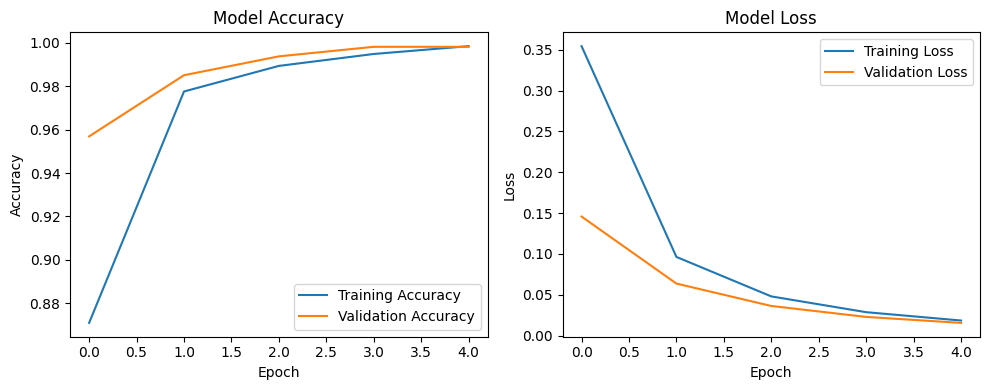
Looking at our training results after 5 epochs, we can observe:
The model achieved excellent performance, with final training accuracy of 99.85% and validation accuracy of 99.82%.
Both training and validation loss steadily decreased across epochs, indicating consistent learning.
Validation metrics consistently tracked close to training metrics, suggesting the model generalizes well rather than memorizing the training data.
Let’s visualize our training progress before moving on:
>>> import matplotlib.pyplot as plt

>>> # Create a simple visualization of training history
>>> plt.figure(figsize=(10, 4))

>>> # Plot training & validation accuracy
>>> plt.subplot(1, 2, 1)
>>> plt.plot([0.8709, 0.9776, 0.9894, 0.9949, 0.9985], label='Training Accuracy')
>>> plt.plot([0.9569, 0.9851, 0.9938, 0.9982, 0.9982], label='Validation Accuracy')
>>> plt.title('Model Accuracy')
>>> plt.ylabel('Accuracy')
>>> plt.xlabel('Epoch')
>>> plt.legend()

>>> # Plot training & validation loss
>>> plt.subplot(1, 2, 2)
>>> plt.plot([0.3543, 0.0964, 0.0481, 0.0288, 0.0186], label='Training Loss')
>>> plt.plot([0.1458, 0.0638, 0.0364, 0.0230, 0.0157], label='Validation Loss')
>>> plt.title('Model Loss')
>>> plt.ylabel('Loss')
>>> plt.xlabel('Epoch')
>>> plt.legend()

>>> plt.tight_layout()
>>> plt.show()
This high performance is promising, but we should verify it on our completely separate test set, which the model has never seen during training. This will give us the most reliable measure of how well our model might perform in real-world scenarios.
Step 4: Evaluate the Model’s Performance on Test Data
The true test of our model’s capabilities comes from evaluating it on our completely separate test dataset. Let’s see how our neural network performs when classifying mushrooms it has never encountered before!
>>> # Make predictions on the test data
>>> y_pred=model.predict(X_test)
For a binary classification problem like our (poisonous vs edible), the model outputs probabilities between 0 and 1 for each sample. Let’s show the first sample’s prediction:
>>> y_pred[0]
array([0.00323989], dtype=float32)
This shows the probability for the first mushroom sample in the test set. The output is a single value between 0 and 1, where:
Values closer to 1 indicate the model is more confident that the sample is poisonous.
Values closer to 0 indicate the model is more confident that the sample is edible.
For example, our output value is 0.00323989, which means that the model is ~99.68% confident that the sample is edible.
The model outputs probability values, but for practical mushroom classification, we need definitive “edible” or “poisonous” predictions. We need to convert these continuous probability values into discrete class labels:
>>> import numpy as np

>>> # Convert probabilities to binary predictions using a threshold of 0.5
>>> y_pred_final = (y_pred > 0.5).astype(int)
This code performs what’s called “thresholding”:
First, we compare each probability to the threshold value (0.5)
If probability > 0.5, the result is True (model thinks it’s more likely poisonous)
If probability ≤ 0.5, the result is False (model thinks it’s more likely edible)
Then, we convert these True/False values to integers (1/0) with
.astype(int)True becomes 1 (poisonous)
False becomes 0 (edible)
The 0.5 threshold represents the decision boundary - the point where the model is equally confident in either class. We could adjust this threshold if we wanted to be more conservative about certain types of errors (e.g., lowering the threshold would classify more mushrooms as poisonous, reducing the chance of missing toxic ones).
Now, let’s visualize the model’s prediction accuracy with a confusion matrix. This will allow us to see how many correct vs incorrect predictions were made using the model above.
>>> from sklearn.metrics import confusion_matrix
>>> import seaborn as sns

>>> # Create confusion matrix
>>> cm=confusion_matrix(y_test,y_pred_final)

>>> # Create visualization
>>> plt.figure(figsize=(10,7))          # Set figure size to 10x7 inches
>>> sns.heatmap(cm,annot=True,fmt='d')  # Create heatmap with annotations and display counts as integers
>>> plt.xlabel('Predicted')             # Label x-axis as 'Predicted'
>>> plt.ylabel('Truth')                 # Label y-axis as 'Truth'
>>> plt.show()                          # Display the plot
Output of the above confusion matrix is as follows:
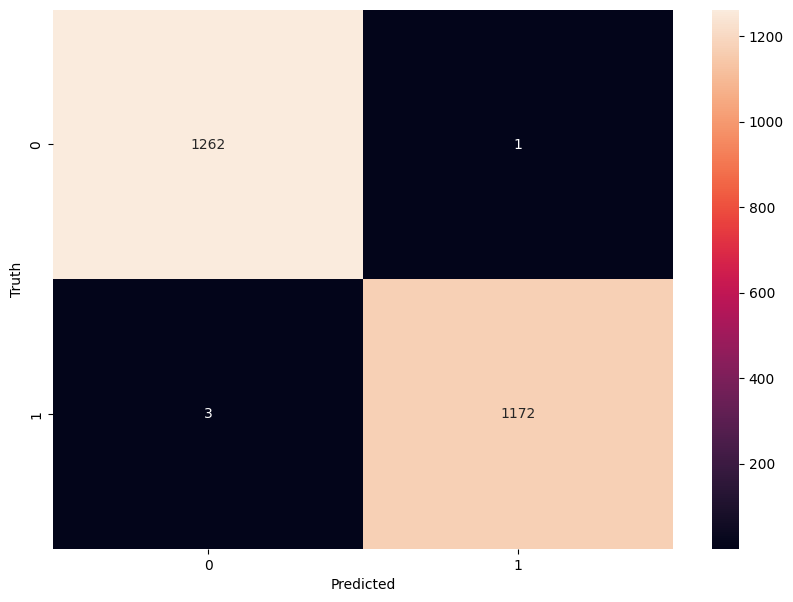
The confusion matrix visualization shows how well our model classifies mushrooms as edible or poisonous. The matrix is a 2x2 grid where:
The y-axis (Truth) shows the actual class of the mushrooms
The x-axis (Predicted) shows what our model predicted
Each cell contains the count of predictions falling into that category
The heatmap coloring provides visual intensity, where lighter colors indicate higher counts
Reading the matrix:
Top-left: True Negatives (TN) - Correctly identified edible mushrooms
Top-right: False Positives (FP) - Edible mushrooms incorrectly classified as poisonous
Bottom-left: False Negatives (FN) - Poisonous mushrooms incorrectly classified as edible
Bottom-right: True Positives (TP) - Correctly identified poisonous mushrooms
Key Classification Metrics
From these confusion matrix values, we can calculate several important evaluation metrics:
Metric |
Definition |
Interpretation for Mushrooms |
|---|---|---|
Accuracy |
\(\frac{TP + TN}{TP + TN + FP + FN}\) |
Percentage of all mushrooms correctly classified |
Precision |
\(\frac{TP}{TP + FP}\) |
When model predicts “poisonous,” how often is it right? |
Recall |
\(\frac{TP}{TP + FN}\) |
Of all poisonous mushrooms, how many did we correctly identify? |
F1-Score |
\(2 \times \frac{Precision \times Recall}{Precision + Recall}\) |
Harmonic mean of precision and recall; useful when you need to balance both |
Specificity |
\(\frac{TN}{TN + FP}\) |
Of all edible mushrooms, how many did we correctly identify? |
Thought Challenge: Which prediction metric is most important for this model? Why?
For mushroom classification, false negatives (bottom-left) are particularly concerning as they represent poisonous mushrooms that were incorrectly classified as edible.
Recall measures a model’s ability to correctly identify all true positives within a dataset, minimizing false negatives. Therefore, recall is the most important metric for this model.
Let’s also print the full classification report of this model using code below
>>> from sklearn.metrics import classification_report
>>> print(classification_report(y_test,y_pred_final, digits=4))
              precision    recall  f1-score   support

           0     0.9976    0.9992    0.9984      1263
           1     0.9991    0.9974    0.9983      1175

    accuracy                         0.9984      2438
   macro avg     0.9984    0.9983    0.9984      2438
weighted avg     0.9984    0.9984    0.9984      2438
The accuracy of our model is 99.84%, so 99.84% of the time, this model predicted the correct label on the test data.
Thought Challenge: Did we build a successful model? Why or why not? Is there anything we can do to improve the model?
Did we build a successful model?
By standard performance metrics, our model is remarkably successful:
Accuracy of 99.84% on the test set
Recall of 99.74% for poisonous predictions
Precision of 99.91% for poisonous predictions
F1-score of 99.83% for poisonous predictions
Why it’s successful:
The model efficiently learned the patterns distinguishing edible from poisonous mushrooms
The architecture, despite being simple (just one hidden layer), was sufficient for this task
The dataset is well-structured with clear categorical features that strongly correlate with mushroom edibility
However, there are important considerations:
In a real-world mushroom classification system, even our 99.74% recall means that approximately 3 out of 1000 poisonous mushrooms were misclassified as edible. For a life-critical application like mushroom toxicity detection, this error rate is still too high.
Potential improvements:
Domain-specific threshold adjustment: Lower the classification threshold from 0.5 to a more conservative value (e.g., 0.3) to reduce the likelihood of false negatives (missing poisonous mushrooms)
More sophisticated architecture: Try deeper networks or different architectures that might capture more subtle patterns
Ensemble methods: Combine multiple models to reduce the chance of missing poisonous mushrooms
Cost-sensitive learning: Explicitly penalize false negatives (missing poisonous mushrooms) more heavily during training
Uncertainty estimation: Add methods to quantify prediction uncertainty, so users know when to seek additional verification
Real-world deployment considerations:
Even with an improved model, it would be ethically questionable to deploy such a system as the sole decision-maker for mushroom consumption. It should be presented as a tool to assist experts rather than replace human judgment, especially for life-critical decisions.